As part of the WATT THE HACK hackathon, my teammates and I participated in the Nomadic drone challenge - we met the same morning for the first time, brainstormed ideas and came up with the following solution. We didn't win but I'm proud of what we built in less than a day.

The challenge

A storm has just passed over a section of the Bavarian overhead grid. Some areas have lost power and the operator needs to know where to look first. The toolkit is five mobile sensor packages, basically drones that sit on power lines. Each one can fly for 30 minutes, then has to charge for 3 hours, and it can only charge on a live line.

What we had to start from was a map of line segments and six fictional storm reports ("a flash was seen somewhere around here", "trees in the area", confidence: low to medium). The reports are vague and possibly wrong. The questions: what do you measure, where do the drones start, how do they move as information comes in, and when is the evidence strong enough to send a repair crew?

Our approach

The whole system rests on one data structure: a belief per cell and fault type. We cut every line into ~500 m cells and keep, for each cell and each fault type (vegetation, sag, ice, galloping, hotspot, broken conductor), the probability p_t that this fault is there. A cell's risk is the probability that any fault is there:

risk(cell) = 1 − Π_t (1 − p_t)

(As you can see, we take the product of the probabilities that a fault of type t is not there for each type - this assumes that the faults are independent of each other, which definitely is a simplification, e.g. ice makes the line heavier causing sag).

Everything else is either building this belief, updating it, or deciding where to collect evidence next.

The prior: turning vague inputs into a risk map

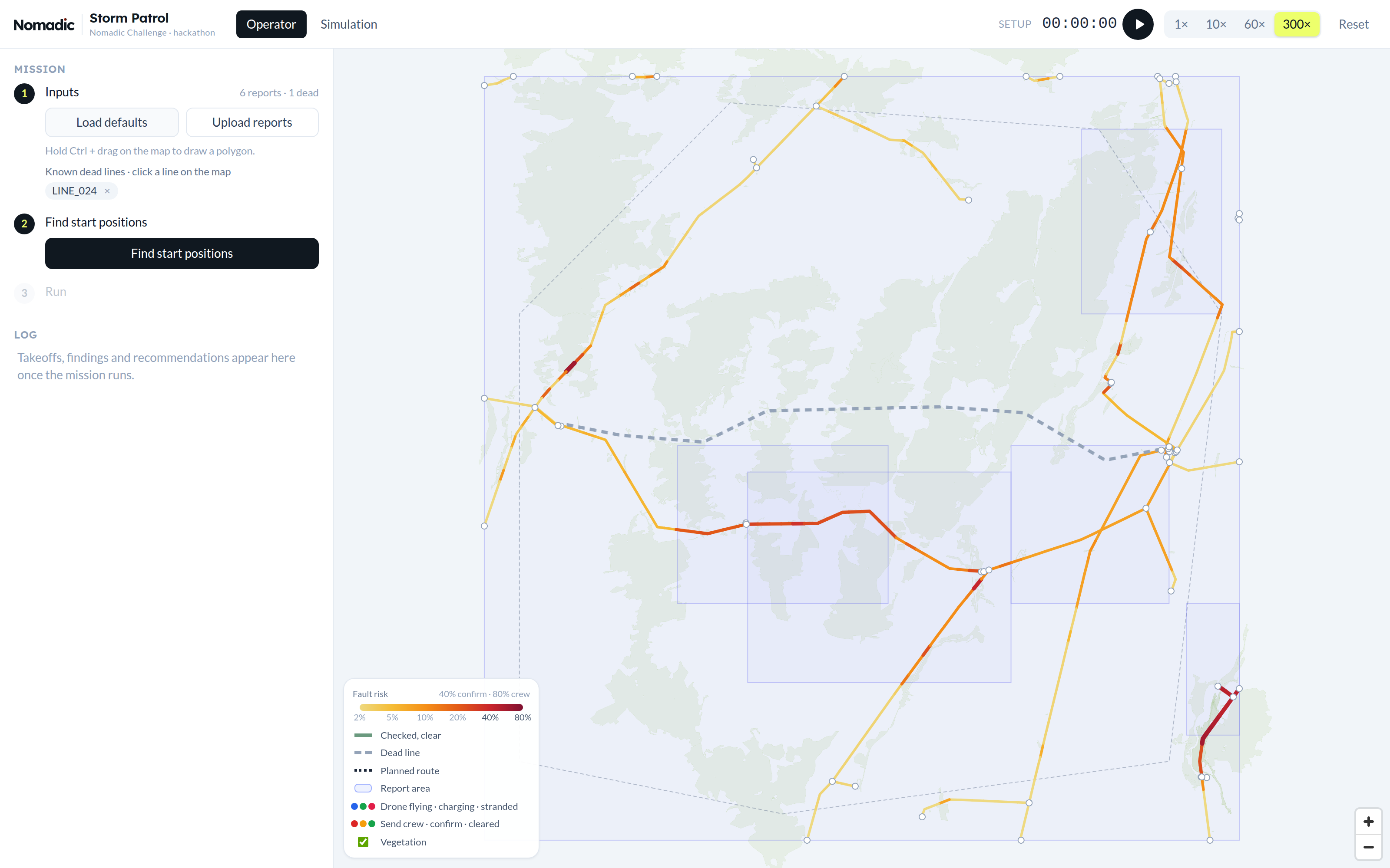
Before any drone flies we combine everything we know into a prior:

• Reports: Each report adds confidence × type weight × spread to the cells its polygon touches.
  • The spread factor min(1, 10 / n_cells) matters: a report covering the whole region says almost nothing about any single cell, while a report covering only 4 cells says a lot about each.
  • Here is another simplification we made - there's one constant weight per fault type, no matter what a report mentions about it. In reality one report can point strongly at a hotspot and another only weakly, but once a type is assigned to a report, we treat both the same. A better approach would be to pre-screen each report with an LLM and estimate a weight for every fault type from its content.
  • Our constant weights were hand-tuned guesses.
• Vegetation: We exported forest and tree rows from OpenStreetMap and compute how much of each cell's 30 m buffer is wooded. Lines through forest are where trees fall on lines.
• Storm footprint: Wind-driven fault types get damped outside the storm area.
• Known dead lines: A dead line might have a broken conductor somewhere along it, and lines sharing a node with it get a small bump. It's deliberately small, because sharing a node on the map doesn't prove an electrical connection (as stated in task).
• Other sources: If other data sources are available (satellite imaging, weather data ...) they can be simply included in this step.

Valuing cells by expected detections

To decide on starting positions and flight routes, we need to value cells somehow, so we used one common unit: expected number of detections. Each cell gets two values: one for the value of flying over it and one for landing on it. This is because some faults are easy to detect from the air (camera -> vegetation, thermal camera -> hotspot) while others can only be found landed (IMU -> sag, vibration -> galloping, ...)

value_air(cell) = Σ_t p_t · p_detect_air_t
value_landed(cell) = Σ_t p_t · p_detect_landed_t

p_t is the probability that a fault of type t is in that cell (derived from prior and previous inspections) p_detect_METHOD_t is the probability that we detect a fault of type t with METHOD

This will allow us later to evaluate the value of a flight easily.

Start positions

Finding the right start positions is one of the most important points - if you choose the wrong ones a lot of time is spend at the wrong places. Therefore our approach works as follows: Start positions are picked greedily, one drone at a time. For each drone we take the best candidate cells (on lines we're confident are live, at least 3 km from other drones) and actually plan the first flight from each one. The winner is the candidate cell and flight that results in the most expected detections, plus a bonus for landing near cells only landed sensors can check. Cells covered by an earlier drone's flight keep only 15 % of their value, so the next drone goes somewhere else.

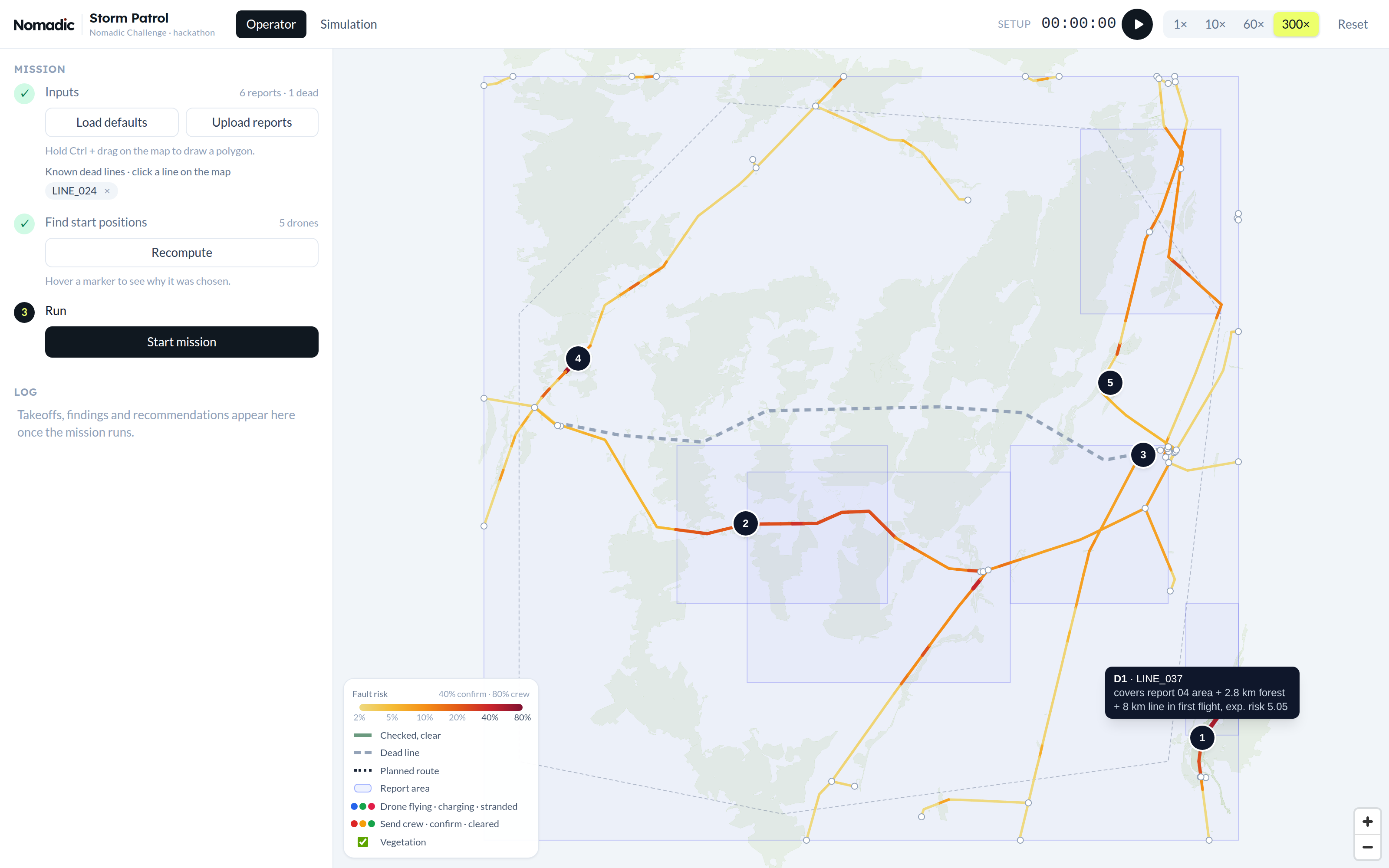
Greedy isn't optimal, but it's fast. The tooltip in the app shows the reasoning for this position to the operator.

Determining flight paths - the orienteering problem

Computing the optimal mission would be expensive in time and compute so we planned from flight to flight. And also on the flight level, we didn't go for the fully optimal flight but built it greedily from shorter sections aka runs - stretches flown along a single line, inspecting every cell on the way and connected through transits. Why? Our platform allowed us to simulate the whole scenario with speeds up to 300x, so decision making needed to be quick and explainable.

So the planner starts from the drone's position and adds the run with the best value / time (the transit to get there counts as time), then the best next run from where that one ends, and so on. A run is only allowed if the drone can still reach a landable cell afterwards, including 3 min for landing and a 5 min reserve. When no run fits anymore, the flight ends with the landing. The reserve is there because a drone might land on a line that turns out to be dead (current ≈ 0), and then it needs enough battery to hop to another one. The landing spot itself is chosen by what can be checked from there: landed-only faults nearby, future flights, and how sure we are the line is live.

The whole flight is planned at take-off and the drone sticks to it, with one exception: if it sees something that needs confirmation, it can drop the rest of its route and land on that cell right away.

Charging is assumed to be linear (3 h for 30 min of flight), and drones take off with a partial charge when a short hop is worth it, for example to confirm a finding.

Updating the belief with Bayes

Every pass over a cell is an observation, and the belief is updated with Bayes' rule using the sensor's detection and false-positive rates:

no detection:  p' = p·(1 − p_d) / (p·(1 − p_d) + (1 − p)·(1 − p_fp))
detection:     p' = p·p_d / (p·p_d + (1 − p)·p_fp)

A clean pass lowers the belief without zeroing it: a camera with pd = 0.85 takes a 30 % vegetation probability down to about 6.5 %. A detection pushes it up sharply. Only the fault types the sensor can see are updated, so a clean flyover says nothing about galloping, which can only be detected when landed. Risk and value are then recomputed from the updated beliefs, and the next flight is planned on the new map. That's the whole feedback loop: observe → update → re-plan. Line status (live or dead) is a belief too, updated for the complete line by landings (the current sensor is certain).

Two places where we deliberately bend pure Bayes:

• Sensor confidence. While Bayes follows a binary approach: detection vs no-detection, we included the sensor's confidence into our model: 'I'm 60% sure that there is a vegetation fault'. The confidence rating is taken from the simulation: a real detection from the air gets a confidence between 0.6 and 0.95, and a landed one between 0.85 and 0.99, while a false positive gets a confidence between 0.3 and 0.7. We apply this confidence as follows:

  p' = confidence · posterior + (1 − confidence) · p
  

  As a result, a single unsure detection lands in "needs confirmation" (40–80 %) instead of jumping straight to "send crew". A drone then confirms it, either by a second look or by landing on the cell right away.

• Explaining away. A report describes one event in its area. When building the prior, each of its cells gets a sizeable share of the report, cells in small report areas even the full amount (see the spread factor above). After a clean pass every cell keeps a bit of that evidence, so the area as a whole still looks risky and drones keep coming back. To counter this, once a report area has been fully inspected without a finding, we reset those cells to their prior without that report, which treats the report as a false alarm.

The app

We built this as a web app: a FastAPI backend that holds the planner and simulation, and a React + MapLibre frontend with two views:

The operator view is a three-step flow: load reports (or draw a report area on the map) and mark known dead lines, compute start positions, start the mission. From there the operator watches the drones fly. Line colours show the current risk, green means checked and clear, and the sidebar shows what every drone is doing.

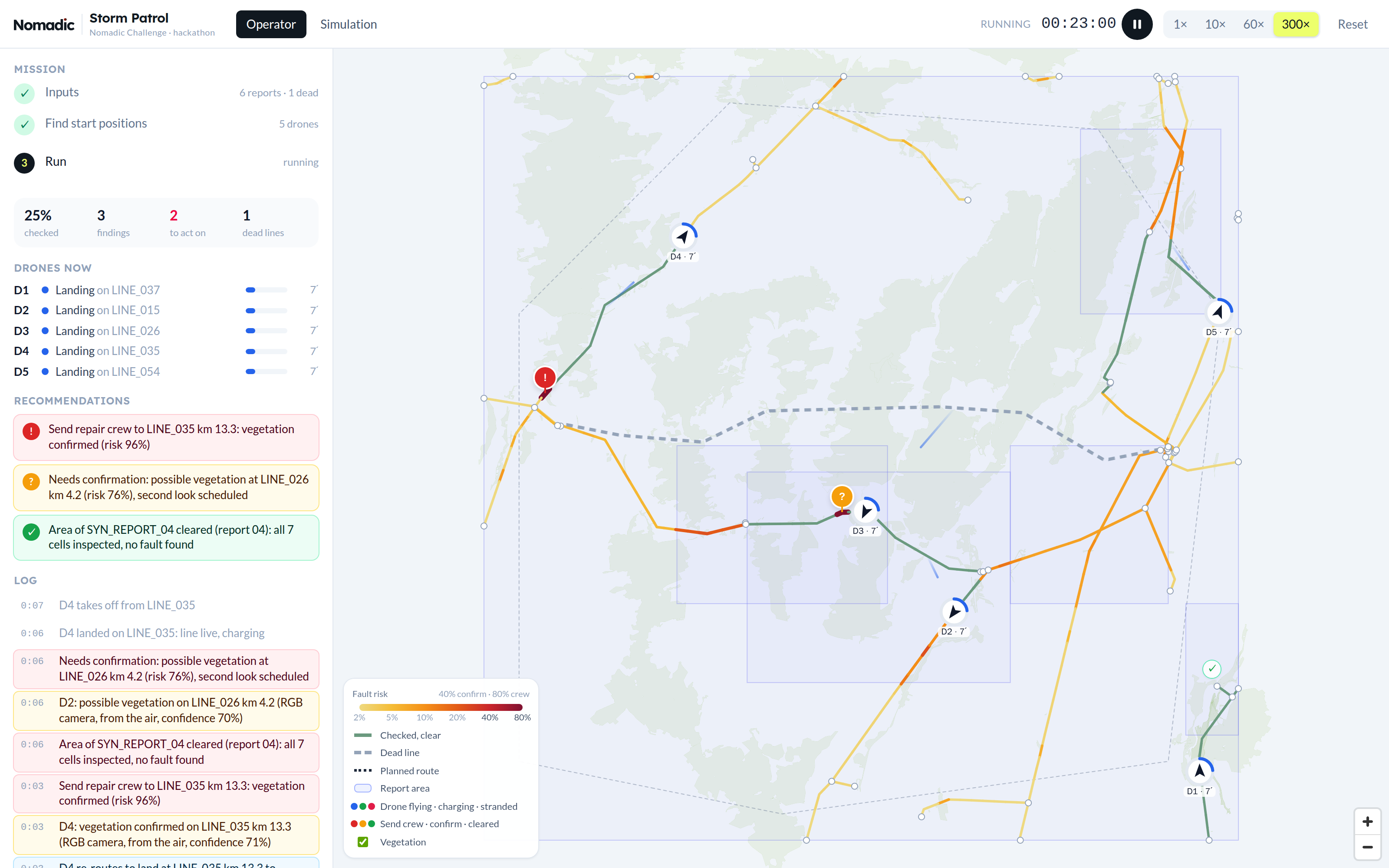
The output that matters is the recommendations list. It turns beliefs into actions with fixed thresholds: send repair crew (confirmed, risk > 80 %), needs confirmation (40–80 %, a second look is already scheduled), inspect from the ground (a dead line was flown completely without finding the cause), and area cleared (a report area fully inspected, risk below 40 %). Clicking an entry flies the map there and opens a short report with the evidence behind it.

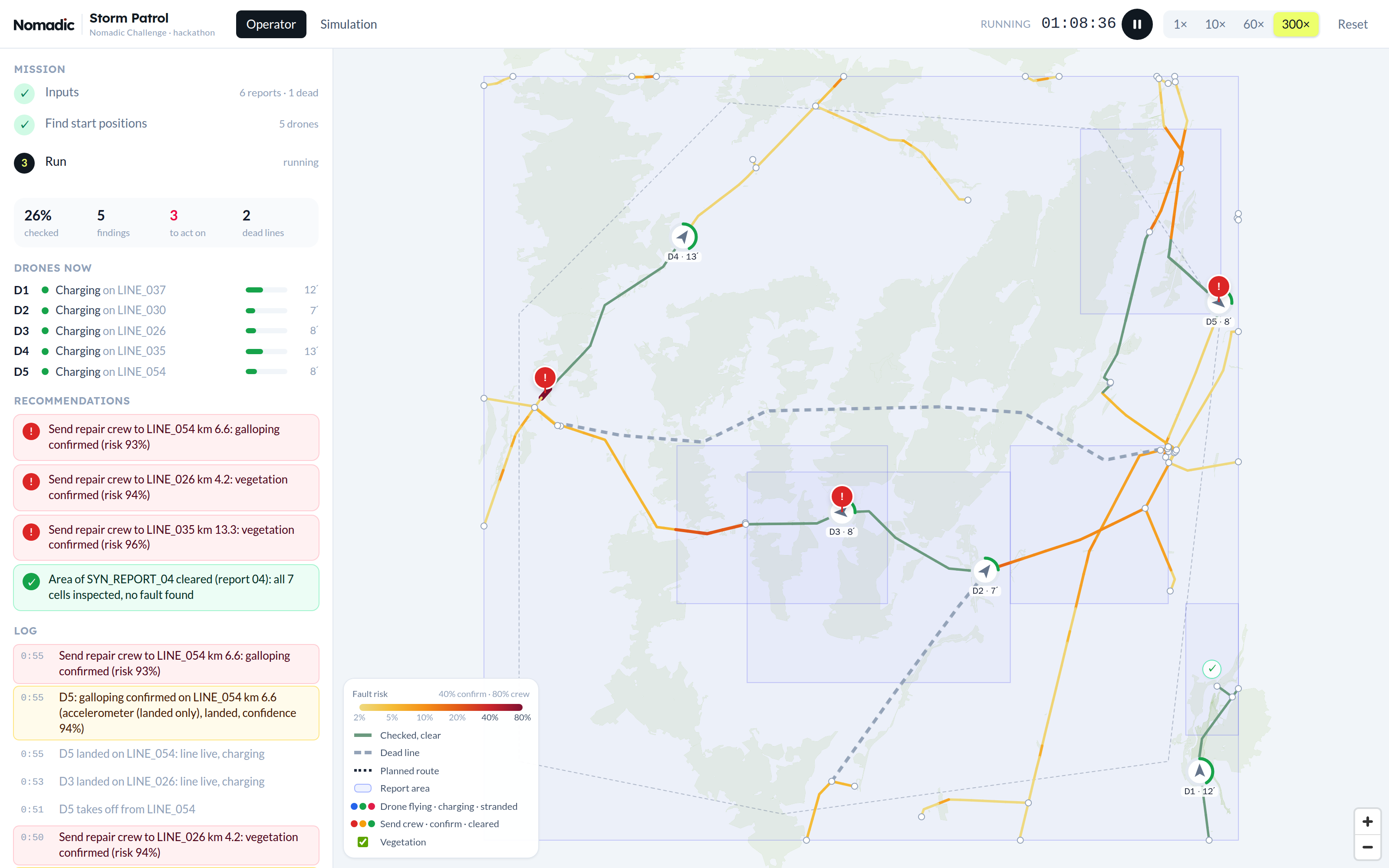
Since we had no real drones, the app includes a simulation view. It holds the hidden ground truth: where the faults actually are, which lines are secretly dead, and the sensor detection and false-positive probabilities. The simulator rolls the dice for every pass and only sends the planner observations, the same way real drones would. The planner code never imports the simulator, so it can't cheat. Runs are seeded, so the same scenario always gives the same run, which made debugging much easier.

Limitations

Everything is synthetic: the reports, the faults and the sensor probabilities are made up, and the planner weights are tuned by hand. Wind isn't modelled (no flight ban in gusts, no effect on battery), lines are treated as electrically independent, and the drones fly straight lines with no airspace or terrain constraints. The greedy planner has no optimality guarantee. Still, the core idea of keeping a belief per fault type, valuing every action by expected detections and updating it after every observation turned a pile of vague reports into decisions an operator can follow, and it's all explainable down to the single number behind each choice.